Parametric Curve Equations

by Tuğrul Yazar | September 19, 2021 00:39

The parametric curve[1] equations are good examples to demonstrate the bridge between computer-aided design and mathematics. Although useless and pointless, it is a good exercise to extract the curve equations. In this Rhino Python[2] code, I present a generalized equation extractor for Rhino. Rhino curves are good examples de Casteljau[3] and Bézier[4] curves. You can see the mathematical underpinnings of Rhino curves with this exercise:

from math import *
import rhinoscriptsyntax as rs
p = []
f = g = h = ""
d = rs.GetInteger("Enter degree ",3,1,7)
for i in range(d + 1):
	point = rs.GetPoint("Specify control point #"+str(i + 1))
	p.append(point)
	rs.AddPoint(point)
for i in range(d + 1):
	c = factorial(d)/(factorial(i)*(factorial(d-i)))
	f += "("+str(c)+"*((1-t)**("+str(d)+"-"+str(i)+"))*(t**"+str(i)+")*"+str(p[i][0])+")+"
	g += "("+str(c)+"*((1-t)**("+str(d)+"-"+str(i)+"))*(t**"+str(i)+")*"+str(p[i][1])+")+"
	h += "("+str(c)+"*((1-t)**("+str(d)+"-"+str(i)+"))*(t**"+str(i)+")*"+str(p[i][2])+")+"
f += "0"; g += "0"; h += "0"
print("These are the three (x,y,z) parametric equations of the curve")
print("f = "+f)
print("g = "+g)
print("h = "+h)
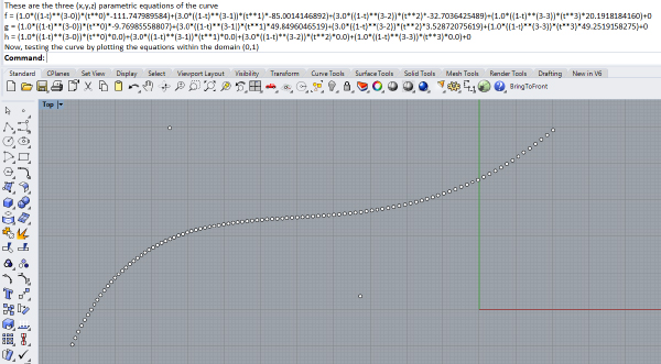
print("Now, testing the curve by plotting the equations within the domain (0,1)")
for i in range(0,100):
	t = i / 100
	point = [eval(f), eval(g), eval(h)]
	rs.AddPoint(point)

This code asks the user the degree of the curve. By default, Rhino’s curves are degree 3. Therefore, our default value is 3. After that, the script asks the user to specify the control points of the curve. The number of control points is always degree+1. More control points will require the decomposition of the curve into degree 3 spans. Maybe, I will post something about this later. After getting these data, the script starts building the equations.

The standard parametric curve has three equations; f, g, and h. These equations control the x, y, and z coordinates of the points on the curve. These equations are independent of each other, but all of them include one variable called t. This is the parameter, which is generally between 0 and 1. You need to plug the t value into these equations and calculate the x, y, and z coordinates. We build these equations as string values in the script.

Overall, we are constructing the Bernstein polynomial here. The line with “factorial” functions is called the “binomial” function. The other lines utilize the general Bernstein polynomials by plugging the coordinate values, the binomial coefficient, the degree, and other stuff. If you are interested in this part, I recommend looking at here[5]. Finally, the script displays the three parametric curve equations and uses them to draw 100 points for verification.

Source URL: https://www.designcoding.net/parametric-curve-equations/