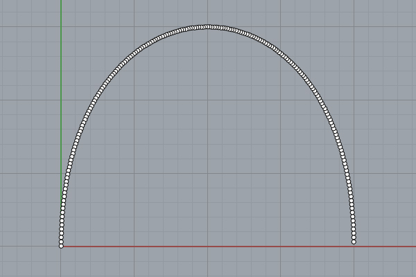
Cubic Bézier Curve with Rhino Python

by Tuğrul Yazar | April 30, 2018 23:39

Below is the Python code you can run in Rhino, that draws a cubic Bézier curve [1](degree 3). As you can see, the Rhino Python[2] code is very slow and inefficient because we calculate every point with lots of computations. Instead, we can use the spline formulae to make this quicker but I wanted to show that the mathematical construction is parallel to the geometric one. This is a nested set of linear interpolations. In fact, the linterp function in the code is the key to this method.

import rhinoscriptsyntax as rs

## Degree 3 Beizer Curve

def linterp(p1,p2,t):
	tx = p1[0] + (p2[0] - p1[0]) * t
	ty = p1[1] + (p2[1] - p1[1]) * t
	return (tx,ty,0)

p1 = (0,0,0)
p2 = (0,20,0)
p3 = (20,20,0)
p4 = (20,0,0)
t = 0

while t <= 1:
	t1 = linterp(p1,p2,t)
	t2 = linterp(p2,p3,t)
	t3 = linterp(p3,p4,t)
	t4 = linterp(t1,t2,t)
	t5 = linterp(t2,t3,t)
	t6 = linterp(t4,t5,t)
	rs.AddPoint(t6)
	t = t + 0.005

The code is a while loop, iterating a number (t) from 0 to 1 by 0.005 at each step. You can modify these initial values and see their effects. If you increase the gap between the domain (0 and 1), you will “extend” the curve. Similarly, if you decrease it, you will “trim” the curve. You can change the increment to generate more or fewer points and make it faster but less correct. Be careful not to crash by going into an infinite loop in this while block. To draw the cubic bézier curve, we need four control points. These are p1, p2, p3, and p4 in the code. The while loop calls linear interpolation at each iteration to calculate one point. The linear interpolation, in fact, is a vector addition and multiplication operation. As you can see, Rhino Python handles coordinates as vectors successfully.

In the future, I am planning to study this and similar codes more. This helps me understand the mathematics behind computer-aided design at a fundamental level.

Source URL: https://www.designcoding.net/drawing-cubic-bezier-curve-with-rhino-python/